
Simulation Post-processing
The Simulation Post-processing task is designed to perform statistical calculations from simulations (stored in a macro variable). It can be applied to simulation results produced by any simulation algorithm and supports both numerical and categorical simulation variables.
For numerical simulations, the task computes classical statistical indicators describing the distribution of simulated values, such as the average of simulations, confidence intervals, probability of exceeding a threshold, etc. The tool offers the same post-processing results as in Simulations.
For categorical simulations, it derives statistics based on the distribution of categories across realizations. The tool offers the same post-processing results as in Pluri-Gaussian Simulations, Sequential Indicator Simulations or Multiple-Point Statistics.
This task allows computing additional statistics without recomputing the entire set of simulations, which can be time consuming.
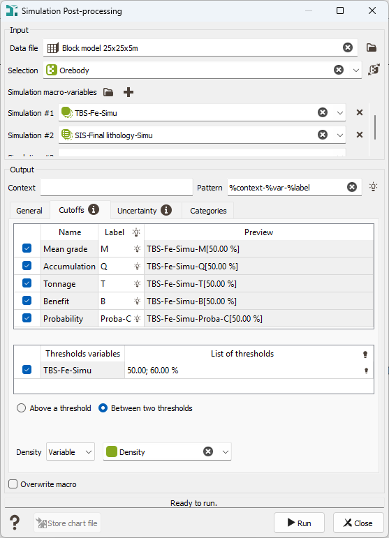
Input
- Click the directory icon to pop up a Data Selector and select the input Data table which contains the simulation results. The input file is mainly a Grid file, but it can be of any type, Sub-blocks, Points, etc. This data table can also be defined by a simple and quick drag-and-drop from the Data tab. A Selection variable may be specified. In this case, only the samples defined by the selection (i.e. samples where the value of the selection is equal to 1) will be considered for the calculations. This selection can also be defined by a categorical variable.
- Then define the Simulation set to be considered for the statistical calculations. It can be a numerical macro variable or a categorical macro variable, depending on the type of simulation performed. You can select several simulation sets. In this case, the same kind of statistics will be calculated on output for each type of simulations.
Output & Parameters
The objective of the Pattern (and Context) parameter is to help the definition of output results names. You can edit this pattern and define the name of your choice. Click on  to retrieve the default pattern: %context-%var-%label
The Label section is editable by a double-click for modification. The Preview enables you to see the final name associated to each output result (for the first simulation set).
You may then specify several output variables grouped in four different tabs:
-
General: Under this tab, you will find main statistics (mean value, standard deviation, variance, coefficient of variation, minimum or maximum of the realizations of the target variable and quantiles) of numerical simulations.
-
Mean: gives the mean value of the set of simulations on each cell or block of the grid.
-
Standard Deviation / Variance: gives the standard deviation / variance of the set of simulations on each cell or block of the grid.
-
Coefficient of variation: corresponds to the ratio of the standard deviation to the mean.
-
Minimum: gives the minimal envelope of the set of simulations on each cell or block of the grid (that means that, for each node of the grid, the program selects the simulation which is the smallest one. It could be different from one node to another).
-
Maximum: gives the maximal envelope of the set of simulations on each cell or block of the grid (that means that, for each node of the grid, the program selects the simulation which is the biggest one. It could be different from one node to another).
-
Quantiles: enables the calculation of different quantiles for each cell or block of the grid. For a given quantile p, the quantile map displays the value for which there is p% of chance (i.e. p% of the simulations) that the real value z is smaller than this value. In this application, a quantile is always one of the simulation values of the macro variable.
Click
 Edit to pop up the Value Definition window and customize the list of quantiles.
-
-
Cutoffs: Under this tab, you will find results associated with threshold(s) and applied on numerical simulations.
-
The two following options only appear if we consider several variables (with a multivariate geostatistical set or selecting several sets of simulations):
- Thresholds on main variable: Select this option if you want to apply threshold(s) to one of your simulated variables only. Other variables will not consider threshold(s).
- Thresholds per variable: Select this option if you want to apply different threshold(s) to each simulated variable.
When defining several thresholds, the two following options appear:
- Above a threshold: Select this option if you want to consider simulated values greater or equal to a defined threshold.
- Between two thresholds: Select this option if you want to consider simulated values within an interval defined by two thresholds, i.e. values greater or equal to the lowest threshold and strictly lower to the greatest threshold.
Click
Edit to pop up the Value Definition window and customize the list of thresholds. -
Mean grade: for each node of the grid, the program computes the average value of the simulated values greater than or equal to the defined threshold or within the two defined thresholds.
-
Accumulation: for each node of the grid, the program calculates the sum of the simulated values which are greater than or equal to the defined threshold or within the two defined thresholds, multiplied by the area or the volume of the cell. This sum is then divided by the total number of simulations.
In 3D, a Density factor is also applied to compute masses. The density can be a constant value or defined by a variable. In this last case, the selected variable should be associated with a Mass density unit class.
In 2D, a Thickness factor is also required. The thickness can be a constant value or defined by a variable. In this last case, the selected variable should be associated with a Length unit class.
Depending on the type of the variable, the result can be homogeneous to a tonnage for a grade, or a volume for a thickness in 2D for example.
-
Tonnage: corresponds to the rock quantity (in weight) where the simulated value of the variable is greater or equal to the cutoff value (or within the interval in the case we consider two thresholds).
-
Benefit: corresponds to the difference between the metal quantity you should obtain with the calculated grade and the metal you would have obtained if the blocks had the exact cutoff value, so a value lower than the grade value.

-
Probability: for each node of the grid, the program computes the number of simulations whose the value is greater than or equal to the defined threshold or within the two defined thresholds. When normalizing this value to the total number of simulations, this gives a probability (between 0 and 1) for the node to exceed the defined threshold.
-
-
Uncertainty: This tab is reachable if a numerical simulation set has been selected.
-
Confidence interval width: the confidence interval map represents the width of the interval which contains the real value at a given confidence level. For each node of the grid, simulated values are sorted in increasing order to compute quantiles (a quantile is always one of the simulation values of the macro variable). The p% confidence interval is based on the computation of two symmetric quantiles:

Click
Edit to pop up the Value Definition window and customize the list of confidence intervals. -
Relative-to-mean estimation error: corresponds to the ratio of the confidence interval width to the mean multiplied by two:
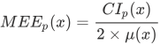
-
Relative-to-median estimation error: corresponds to the ratio of the confidence interval width to the median
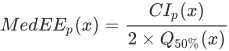
-
Tolerance width: combined with the probability within tolerance variable, this result is used for the Parker's classification.

Click
Edit to pop up the Value Definition window and customize the list of tolerances. By default, the tolerance is set to 15%. -
Probability within tolerance: for each node of the grid, the program computes the number of simulations whose value lies in the interval defined by the mean value more or less the tolerance. When normalizing this value to the total number of simulations, this gives a probability (between 0 and 1).

-
-
Categories: This tab corresponds to the post-processing of categorical simulations and by consequence, it is reachable if a categorical simulation set has been selected.
-
the Probabilities macro variable with an index for each lithotype defined earlier (each category of your lithotype variable): for each node of the grid and for each lithotype, the program computes the number of simulations belonging to this lithotype. When normalizing this value to the total number of simulations, this gives a probability (between 0 and 100 with a % unit) to be in the defined lithotype.
-
the Most probable lithotype categorical variable will store the most represented category/lithotype of the simulations (i.e. the category/lithotype with the highest proportion).
-
the Least probable lithotype categorical variable will store the least represented category of the simulations (i.e. the category with the smallest proportion).
-
the Proba diff with input proportions macro variable with an index for each category defined earlier (each category of your lithotype variable): absolute value of the difference between the input proportions (global or local) and proportions/probabilities calculated from the simulations.
Note: This output can only be computed if the input proportions are available in the simulation results. If this information is not available, the variable cannot be generated.
See Default proportions for more information about how these proportions are retrieved.
-
the Entropy numerical variable will represent the average level of uncertainty inherent to the variable’s possible outcomes. It is calculated by the following formula:
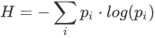
where pi is the probability (between 0 and 1) of the lithotype i and log represents the logarithm base 2.
-
the Corrected most probable lithotype (Soares): The Soares correction is meant to correct the lithotype probabilities after the simulation by taking into account the global probabilities. Using this algorithm, a new most probable lithotype can be deduced. This algorithm is detailed in:
- Soares (1992): Geostatistical Estimation of Multi-PhaseStructures, Mathematical Geology, Vol. 24, No.2, 149-160.
- Soares (1998): Sequential Indicator Simulation with Correction for Local Probabilities, Mathematical Geology, Vol. 30, No.6, 761-765.
If the Corrected most probable lithotype (Soares) variable is asked to be stored, click the Proportions for correction button to modify the proportion of each input lithotype. By default, the proportions will be the same as the ones defined on input.
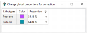
The default proportions are automatically initialized from information available in the simulation results. For categorical simulations generated by Pluri-Gaussian Simulations, Sequential Indicator Simulations or Multiple-Point Statistics, the proportions used during the simulation are stored with the simulation results and are used to initialize the default values.
This information is available only for simulations generated with version 2026.1 or later. If the simulations were generated with an earlier version, this information is not available and the simulation tasks must be run again to store the input proportions.
Note: In Pluri-Gaussian Simulations, input proportions are stored with the simulation results only when the Constant option is used. They are not stored when Variable proportions are used.
If no stored proportions are available, the proportions are estimated from the first realization (first index) of the macro variable. Alternatively, you can initialize the proportions from an existing categorical variable by selecting it using the variable selector.
If multiple categorical macro variables are selected, they must share the same catalog. Otherwise, an error will be generated.
-
Note: When one or more realizations of the macro variable are not defined on a node, this node will not be taken into account in the calculations. Statistics are calculated on the same number of nodes for all the realizations.
- As some results are saved in macro variables, these ones can be overwritten if they already exist by checking the Overwrite macro option. Otherwise, results will be appended (i.e. new indices will be added in the existing macro variable).
- At the end of the run, statistics on the output variables are printed in the Messages window. You can click on the Store chart file button to save the statistics table in a Chart File.
